Срок окупаемости капитальных вложений, формула и примеры

Простой срок окупаемости проекта

Что это такое и для чего он нужен

Простой срок окупаемости проекта – это период времени, за который сумма чистого денежного потока (все деньги которые пришли минус все деньги которые мы вложили в проект и потратили на расходы) от нового проекта покроет сумму вложенных в него средств. Может измеряться в месяцах или годах.

Данный показатель является базовым для всех инвесторов и позволяет сделать быструю и простую оценку для принятия решения: вкладывать средства в бизнес или нет.  Если предполагается среднесрочное вложение средств, а срок окупаемости проекта превышает пять лет – решение об участии, скорее всего, будет отрицательным. Если же ожидания инвестора и срок окупаемости проекта совпадают – шансы на его реализацию будут выше.

В случаях, когда проект финансируется за счет кредитных средств – показатель может оказать существенное влияние на выбор срока кредитования, на одобрение или отказ в кредите

Как правило, кредитные программы имеют жесткие временные рамки, и потенциальным заемщикам важно провести предварительную оценку на соответствие требованиям банков

Как рассчитывается простой срок окупаемости

Формула расчета показателя в годах выглядит следующим образом:

PP=Ko / KFсг, где:

• PP – простой срок окупаемости проекта в годах;
• Ko – общая сумма первоначальных вложений в проект;
• KFсг – среднегодовые поступления денежных средств от нового проекта при выходе его на запланированные объемы производства/продаж.

Данная формула подходит для проектов, при реализации которых соблюдаются следующие условия:

• вложения осуществляются единовременно в начале реализации проекта;
• доход нового бизнеса будет поступать относительно равномерно.

Пример расчета

Пример №1

Планируется открытие ресторана с общим объемом инвестиций в 9 000 000 рублей, в том числе запланированы средства на покрытие возможных убытков бизнеса в течение первых трех месяцев работы с момента открытия.

Далее запланирован выход на среднемесячную прибыль в размере 250 000 рублей, что за год дает нам показатель в 3 000 000 рублей.

PP = 9 000 000 / 3 000 000=3 года

Простой срок окупаемости данного проекта равен 3 годам.

При этом данный показатель необходимо отличать от срока полного возврата инвестиций, который включает в себя срок окупаемости проекта + период организации бизнеса + период до выхода на запланированную прибыль. Предположим, что в данном случае организационные работы по открытию ресторана займут 3 месяца и период убыточной деятельности на старте не превысит 3 месяцев

Следовательно, для календарного планирования возврата средств инвестору важно учесть еще и эти 6 месяцев до начала получения запланированной прибыли

Пример №2

Рассмотренный ранее пример является наиболее упрощенной ситуацией, когда мы имеем единоразовые вложения, а денежный поток одинаков каждый год. На самом деле таких ситуаций практически не бывает (влияет и инфляция, и неритмичность производства, и постепенное увеличение объема продаж с начала открытия производства и торгового помещения, и выплата кредита, и сезонности, и цикличность экономических спадов и подъемов). 

Поэтому обычно для расчета сроков окупаемости делается расчет накопительного чистого денежного потока. Когда показатель накопительно становится равным нулю, либо превышает его, в этот период времени происходит окупаемость проекта и этот период считается простым сроком окупаемости. 

Рассмотрим следующую вводную информацию по тому же ресторану:

Статья	1 год	2 год	3 год	4 год	5 год	6 год	7 год
Инвестиции	5 000	3 000
Доход		2 000	3 000	4 000	5 000	5 500	6 000
Расход		1 000	1 500	2 000	2 500	3 000	3 500
Чистый денежный поток	— 5 000	— 2 000	1 500	2 000	2 500	2 500	2 500
Чистый денежный поток (накопительно)	— 5 000	— 7 000	— 5 500	— 3 500	— 1 000	1 500	4 000

На основании данного расчета мы видим, что в 6 году показатель накопительного чистого денежного потока выходит в плюс, поэтому простым сроком окупаемости данного примера будет 6 лет (и это с учетом того, что время инвестирования составило более 1 года).

Understanding the Payback Period

Corporate finance is all about capital budgeting. One of the most important concepts every corporate financial analyst must learn is how to value different investments or operational projects to determine the most profitable project or investment to undertake. One way corporate financial analysts do this is with the payback period.

The payback period is the cost of the investment divided by the annual cash flow. The shorter the payback, the more desirable the investment.

Conversely, the longer the payback, the less desirable it is. For example, if solar panels cost $5,000 to install and the savings are $100 each month, it would take 4.2 years to reach the payback period.

How do you reduce payback period?

A quicker time to replenish CAC is instrumental to an overall improvement in running your SaaS company and generating revenue. VC Tom Tunguz at Redpoint lauds short payback periods because it means your company has smaller working capital requirements and the ability to grow faster.It is generally considered “healthy” for a SaaS company to have a , although it will vary throughout your company’s lifetime as the various factors that contribute to payback period fluctuate and evolve. However, even though it’s considered acceptable, 12 months is a long time to recoup acquisition costs—which underscores why acquisition is a much less financially efficient growth lever than retention, expansion, and monetization.You need to shorten payback period as much as possible to keep CAC’s drain on your revenue to a minimum.

What is a payback period?

Payback period in capital budgeting is the amount of time it takes for your company to recover the cost of acquiring one customer. For example, a customer that costs $350 to acquire and contributes $25/month, or $300/year, has a payback period of 13.9 months. As time increases, a customer pays back more of their customer acquisition cost (CAC) through their incremental subscription payments.

The example in the graph above shows revenue/spend on the y-axis and time on the x-axis.The time before the company earns back the CAC is shown in red. Eventually, the customer pays back all of their CAC, shown here when the line crossed the x-axis. Then the customer’s payment can go toward the company’s growth. That time period in shown in green. In this example, it takes 15 months for the company to regain CAC.The inverse of payback period is the CAC ratio, or the percentage of sales and marketing spend used to acquired a customer that will be gained back within a year of the customer’s acquisition.

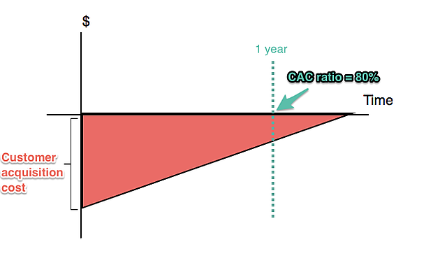
In the example above, the customer pays back their CAC over time, but the time to payback CAC exceeds one year. One year after the customer’s acquisition is marked by the green dotted line. At this point, 80% of the CAC is paid back, meaning the CAC ratio is 80%.

Why is it important to calculate your payback period?

Payback period shows you the efficiency of your acquisition strategies. The shorter your payback period, the more financially efficient your acquisition methods. You need to understand acquisition efficiency to understand how acquiring different types of customers affects your finances and how sustainable your current strategies are in the long term. Keeping a consistently growing cash inflow should be your target from the start: the more accurate your payback method is, the quicker you’ll have money to start reinvesting.Longer-than-ideal payback periods will tell you that you need to make improvements in the areas that affect payback period. The length of your payback period is dependent on:

• • Customer acquisition costs: Subscription-based companies assume the risk of paying CAC upfront and replenishing that spend as . The greater the upfront CAC, the longer it will take to pay it back bit by bit over time.

  • Customer monetization: The size of the increments in which customers pay back their CAC each month (or each year) depends on how you monetize your customers. You may charge them one flat rate, create individualized plans, or scale their pricing according to usage on a value metric. The payment plans that you create for your customers influences the length of the payback period.

Improving any and all of these factors will help you earn back CAC faster, at which point you’ll have future cash flow to invest back into your company and grow.

Что делают из данного вида пластика?

Благодаря высокой химической стойкости и хорошей свариваемости пластик 5 популярен в следующих сферах.

1. Производство упаковки. Из полипропилена получаются прочные гибкие и жесткие тары, различные пленки, пищевые упаковки.
2. Потребительские изделия. Пластик РР пригоден для создания деталей бытовой техники, детских игрушек, мебели.
3. Автомобилестроение. Материал широко используется при производстве корпусов, поддонов, бамперов, приборных панелей и так далее.
4. Волокна и ткани. Из полипропилена получаются прочные ленты, полосы, ремни, объемные непрерывные нити, штапельные волокна, канаты, веревки, шпагаты и прочие тканевые изделия.
5. Медицина. После стерилизации материала паром изготавливают шприцы, медицинские пробирки, компоненты диагностических приборов, бутылок для образцов, ванночек, контейнеров для таблеток и так далее.
6. Промышленность. Листы из пластика 5 пригодны для получения емкостей, в которых будут храниться кислоты, химические реагенты. Также для труб, многооборотной транспортной упаковки и тары.

Формула

Если было принято решение воспользоваться простым методом, то формула здесь будет довольно простой – Т=И/Д:

• Т обозначает период возврата вложенных средств;
• И – величина вложенных финансов;
• Д – сумма прибыли;

Последний фактор представляет собой сумму чистой прибыли и амортизации. Чем меньшим будет итоговый показатель, тем больше вероятности получения довольно значительного дохода, который сможет покрыть не только внесенные средства, но и дать человеку воспользоваться прибылью.

Если человек рассчитывает получить прибыль в течение меньшего срока времени, которое получилось у него в процессе расчетов, то ему желательно отказаться от данного вложения денег.

Методический расчет имеет более сложную формулу, так как здесь приходится учитывать большое количество дополнительных факторов.

В общем виде она выглядит следующим образом: Т=IC/FV:

• Т по-прежнему обозначает в течение какого времени планируется возвратить средства;
• IC – размер вложенных денег;
• FV – доход, который планируется получить в конечном итоге;

При помощи данного способа можно вычислить, насколько обесценятся деньги на момент окончания расчетного периода

Здесь также принимаются во внимание определенные риски, связанные с вложением денежных средств

Помимо инфляции, сюда относятся государственные риски и риски неполучения дохода и, как следствие, непосредственной прибыли. Все эти риски вычисляются в процентной ставке, после чего суммируются, что в конечном счете дает вероятностный процент возвращения денежных средств.

Пример расчета срока окупаемости инвестиционного проекта

Допустим, некий Мистер X покупает машину стоимостью 1 млн. руб. с целью зарабатывать услугами такси. Также предположим: то, что зарабатывает Мистер X как таксист, он кладет в особый конверт. Ну, естественно за минусом расходов, связанных с его бизнесом: минус бензин, минус штрафы и т.п.

Когда в этом конверте накопится 1 млн. руб., Мистер X может с облегчением сказать, что свои деньги он вернул. То есть наступит срок окупаемости.

Пример 1. Срок окупаемости 10 месяцев

Пусть ежемесячная выручка (доход) составляет 100 тыс. руб. Расходы пока не учитываем, Мистер X кладет в особый конверт каждый месяц 100 тыс. руб.

Простой расчет показывает, что 1 миллион наберется за 10 месяцев.

1 000 000 : 100 000 = 10 (месяцев)

Таблица денежных потоков проекта.

Шаг инвестиционного проекта (период по итогам которого осуществляется промежуточное подведение итогов) — 1 месяц.

Денежные потоки на графике:

Расчеты и графики здесь и далее выполнены в excel-таблице «Расчет инвестиционных проектов».

• Линии на графике:
• Красная – расходы
• Синие ромбики – доходы
• Синие треугольники – чистый доход (ЧД) нарастающим итогом.

Видим, что линия ЧД нарастающим итогом проходит через 0 на 10-м шаге, как и показал наш расчет. Это при условии, что расход был только на первом шаге 1 млн. руб.

Пример 2. Срок окупаемости проекта 12.5 месяца

Ежемесячный доход составляет, как и в Примере 1, 100 тыс. руб. Учтем расходы, связанные с инвестиционным проектом: бензин и т.п. Пусть расходы составляют 20 тыс. руб. в месяц. Теперь Мистер X кладет в особый конверт каждый месяц только 80 тыс. руб.

Расчет показывает, что 1 миллион наберется за 12.5 месяцев.

1 000 000 : 80 000 = 12.5

Обратите внимание, что при этом доход не изменился. Таблица денежных потоков

Таблица денежных потоков

Денежные потоки на графике:

На графике видно, что линя ЧД нарастающим итогом проходит через ноль посередине между 12-м и 13-м шагами.

Пример 3. Срок окупаемости …

Ну, и крайний случай: ежемесячный доход составляет, как и в Примере 1, 100 тыс. руб., и расходы составляют 100 тыс. руб. в месяц. Теперь Мистер X ничего не кладет в свой особый конверт.
Вопрос: Когда Мистер X соберет миллион?
Ответ: Никогда.

Обратите внимание, доход опять остался прежним. Таблица денежных потоков

Таблица денежных потоков

Денежные потоки на графике:

How is Payback Period useful to other SaaS metrics?

The payback period is important in measuring the time to pay off your CAC and ACS, while making MRR per customer. Payback period is relevant to:

• • LTV: the lifetime value per customer. You’ll aim to increase LTV over time while decreasing your payback period.

  • LTV:CAC ratio: the return on investment for each customer. Keeping this ratio at 3:1 or higher is a good benchmark for SaaS profitability. But even with a good LTV:CAC ratio, a long payback period will make it difficult for your company to grow quickly

  • ARPU: the average amount of monthly revenue per customer. Increasing ARPU will increase MRR and shorten your payback period, assuming CAC remains the same.

  • MRR: the monthly recurring revenue that is normalized from all recurring items in a subscription. It’s the best way to visualize the cash flow coming from your customers. The more that you grow your MRR, the quicker you’ll reduce your payback period and grow your revenue.

  • MRR Churnthe revenue lost each month from churning customers. It needs to be continuously monitored and reduced to keep your company growing. Significant MRR churn can lengthen the average customer payback period.

The payback period does not account for customer churn nor the time value of money. If you think of the CAC as a loan and the payback period as the loan repayment schedule, you’ll still have to pay the loan even if the customer churns — without the customer’s help.Comparing the payback period for customers acquired through different channels allows you to see which channels are more profitable. You can then focus on the channels that will help your company grow.Read more about building models for SaaS metrics here.

Secrets of companies with relatively short payback periods

, an investor at Spark Capital, admits that there isn’t one universal way to reduce your payback period. Rather, there are general principles that many successful companies with shorter payback periods follow:

«“… A strong brand, great product and continued development, self-service and word of mouth (organic) traction has a lot to do with an efficient sales organization.”

With these principles in mind, you can learn from the with the shortest payback periods and apply them to your growing startup:

1. Focus on organic acquisition, like Shopify. They’ve established a leadership position in a very specific market and built a network within that market. This allows for more acquisitions through referrals and word-of-mouth, which lowers sales and marketing spend.

2. Use a self-service model, like Atlassian. This company has a very specific audience, and by providing the right product to meet that audience’s needs, they don’t need a sales team to sing the product’s praises. Achieving just right product/market fit can help you save massively in sales and marketing spend.

These techniques all help you reduce your sales and marketing spend so that CAC is lower and the payback period is shorter. You can also lower payback period by monetizing your customers better so that they pay back more of their CAC quicker. Below are some of the best techniques from SaaS companies with highly effective customer monetization:

1. 1. Consistently increase expansion revenue, like Front. When you , they’ll pay back their CAC quicker over time.

   2. Upselling customers along a value metric that aligns with usage, like Appcues. As Appcues customers grow and have a greater need for onboarding optimization, they can scale up their plans according to their volume of monthly active users.

   3. Iterating and experimenting with your pricing, like Intercom. There’s no way to know from the get-go what prices will work best to provide the right value match for customers and make sure your company grows and runs efficiently. Don’t be afraid to change your prices to find what works best.

By improving how you monetize your customers, you have the potential to increase customers’ lifetime values and earn more revenue from customers at a faster rate. This means shorter payback periods and higher, faster growth potential.

Advantages and disadvantages of payback method:

Some advantages and disadvantages of payback method are given below:

Advantages:

1. An investment project with a short payback period promises the quick inflow of cash. It is therefore, a useful capital budgeting method for cash poor firms.
2. A project with short payback period can improve the liquidity position of the business quickly. The payback period is important for the firms for which liquidity is very important.
3. An investment with short payback period makes the funds available soon to invest in another project.
4. A short payback period reduces the risk of loss caused by changing economic conditions and other unavoidable reasons.
5. Payback period is very easy to compute.

Disadvantages:

1. The payback method does not take into account the time value of money.
2. It does not consider the useful life of the assets and inflow of cash after payback period. For example, If two projects, project A and project B require an initial investment of $5,000. Project A generates an annual cash inflow of $1,000 for 5 years whereas project B generates a cash inflow of $1,000 for 7 years. It is clear that the project B is more profitable than project A. But according to payback method, both the projects are equally desirable because both have a payback period of 5 years ($5,000/$1,000).

« Prev
Next »

By Rashid Javed (M.Com, ACMA)

Расчет стоимости инвестиций

Этот динамический метод предназначается для подсчета чистой стоимости инвестиций. Под этим параметром понимается различие между суммой денежного потока за срок работы инвестиционного проекта и количеством вложенных в его развитие денежных средств. На основании расчетов принимается решение: если стоимость инвестиций больше нуля, то проект одобряется. Из некоторого числа проектов выбирается наиболее «дорогой».

Чтобы описанный метод расчета показывал корректные значения, должны выполняться такие условия:

• В случае сравнения чистой стоимости одновременно некоторого количества инвестиционных проектов, для них должна использоваться общая дисконтная ставка. Помимо этого, сравниваемые проекты должны быть идентичными по таким параметрам, как продолжительность жизненного цикла и объем вложений.
• Сумма денежных потоков, которая является неотъемлемым параметром при оценивании прибыльности инвестиций в тот или иной проект, должна оцениваться для всего планового периода инвестирования в деятельность бизнес-проекта. Также сумма должна привязываться к конкретным интервалам времени.
• Денежные потоки рассматриваются обязательно отдельно от производственной работы предприятия. Это условие должно выполняться для того, чтобы в ходе анализа оценивались исключительно денежные поступления и платежи, которые прямым образом связаны с осуществлением инвестиционного проекта.

Надо понимать, что рассматриваемый метод позволяет узнать только то, способен ли выбранный вариант инвестиций в работу предприятия положительно сказаться на повышение прибыли компании или дохода самого инвестора. При этом количественную степень такого увеличения оценить не представляется возможным, и это главный недостаток такого метода. Поэтому этот способ рекомендуется дополнять расчетом индекса рентабельности.

Example of Payback Period

Assume Company A invests $1 million in a project that is expected to save the company $250,000 each year. The payback period for this investment is four years—dividing $1 million by $250,000. Consider another project that costs $200,000 with no associated cash savings will make the company an incremental $100,000 each year for the next 20 years at $2 million.

Clearly, the second project can make the company twice as much money, but how long will it take to pay the investment back?

The answer is found by dividing $200,000 by $100,000, which is two years. The second project will take less time to pay back and the company’s earnings potential is greater. Based solely on the payback period method, the second project is a better investment.

3 Examples of Applying the DPP

The numbers used in this example are stemming from the case study introduced in our project business case article where you will also find the results of the simple payback period method. In this analysis, 3 project alternatives are compared with each other, using the discounted payback period as one of the success measures.

Cash Flow Projections and DPP Calculation

The following tables contain the cash flow
forecasts of each of these options. The discount rate was set at 12% and
remains constant for all periods.

Project Option #1

Year	–	1	2	3	4	5	6
Investment and Cost (outflows)	– 5,000	-5,000	-1,000	– 500	– 500	-1,000	-1,000
Benefits and Earnings (inflows)	–	–	3,000	5,000	5,000	4,000	4,000
Net Cash Flow	– 5,000	-5,000	2,000	4,500	4,500	3,000	3,000
Discounting cash flow formula	-5000 / (1 + 12%) ^ 0	-5000 / (1 + 12%) ^ 1	2000 / (1 + 12%) ^ 2	4500 / (1 + 12%) ^ 3	4500 / (1 + 12%) ^ 4	3000 / (1 + 12%) ^ 5	3000 / (1 + 12%) ^ 6
Discounted net cash flow	– 5,000	-4,464	1,594	3,203	2,860	1,702	1,520
Cumulative discounted cash flows	– 5,000	-9,464	-7,870	-4,667	-1,807	– 105	1,415

The relevant rows – the years, the
discounted cash flows and the cumulative discounted cash flows are bolded in
this table. To calculate the DPP, we need to search:

• y (the period preceding the
  period in which the cumulative cash flow turns positive) which is year 5 in
  this example;
• p (discounted value of the cash
  flow of the period in which the cumulative cash flow is => 0) = 1,520, the
  periodic discounted net cash flow of year 6;
• abs(n), the absolute value of
  the cumulative discounted cash flow in period y, which amounts to -105.

Inserting these numbers into the previously
introduced formula [DPP = y + abs(n) / p] looks as follows:

Discounted Payback Period = 5 + abs(-105) /
1520 = 5.07.

Project Option #2

Year	–	1	2	3	4	5	6
Investment and Cost (outflows)	– 15,000	-1,000	-1,000	-1,000	– 500	– 500	-1,000
Benefits and Earnings (inflows)	–	2,500	5,000	5,000	5,000	5,000	5,000
Net Cash Flow	– 15,000	1,500	4,000	4,000	4,500	4,500	4,000
Discounting cash flow formula	-15000 / (1 + 12%) ^ 0	1500 / (1 + 12%) ^ 1	4000 / (1 + 12%) ^ 2	4000 / (1 + 12%) ^ 3	4500 / (1 + 12%) ^ 4	4500 / (1 + 12%) ^ 5	4000 / (1 + 12%) ^ 6
Discounted net cash flow	– 15,000	1,339	3,189	2,847	2,860	2,553	2,027
Cumulative discounted cash flows	– 15,000	-13,661	-10,472	-7,625	-4,765	-2,212	– 185

In this example, the cumulative discounted
cash flow does not turn positive at all. Therefore, a discounted payback period
cannot be calculated. In other words, the investment will not be recovered
within the time horizon of this projection.

Project Option #3

Year	–	1	2	3	4	5	6
Investment and Cost (outflows)	– 3,000	-3,000	-2,500	-1,000	– 500	– 500	– 500
Benefits and Earnings (inflows)	–	–	3,000	4,000	4,000	3,000	3,000
Net Cash Flow	– 3,000	-3,000	500	3,000	3,500	2,500	2,500
Discounting cash flow formula	-3000 / (1 + 12%) ^ 0	-3000 / (1 + 12%) ^ 1	500 / (1 + 12%) ^ 2	3000 / (1 + 12%) ^ 3	3500 / (1 + 12%) ^ 4	2500 / (1 + 12%) ^ 5	2500 / (1 + 12%) ^ 6
Discounted net cash flow	– 3,000	-2,679	399	2,135	2,224	1,419	1,267
Cumulative discounted cash flows	– 3,000	-5,679	-5,280	-3,145	– 920	498	1,765

The cumulated discounted cash flow becomes
positive in period 5. The discounted payback period is calculated as follows:

Discounted Payback Period = 4 + abs(-920) /
1419 = 4.65

Interpretation of the Results

Option 1 has a discounted payback period of
5.07 years, option 3 of 4.65 years while with option 2, a recovery of the
investment is not achieved.

If DPP were the only relevant indicator,
option 3 would be the project alternative of choice. Using the payback period
(without discounting cash flows) would lead to an identical ranking yet option 3
with a PBP of 4.71 years and option 1 with 4.77 years are much closer while in option
2, the investment would be recovered after 5.22 years.

In any case, the decision for a project option or an investment decision should not be based on a single type of indicator. You can find the full case study here where we have also calculated the other indicators (such as NPV, IRR and ROI) that are part of a holistic cost-benefit analysis.

What Is the Difference between Payback Period and Discounted Payback Period?

The discounted payback period has a similar purpose as the payback period which is to determine how long it takes until an initial investment is amortized through the cash flows generated by this asset.

The difference between both indicators is
that the discounted payback period takes the time value of money into account.
This means that an earlier cash flow has a higher value than a later cash flow
of the same amount (assuming a positive discount rate). The calculation
therefore requires the discounting of the cash flows using an interest or
discount rate.

The generic payback period, on the other
hand, does not involve discounting. Thus, the value of a cash flow equals its notional
value, regardless of whether it occurs in the 1st or in the 6th year. This may fit for the purpose of many high-level analyses. However, it
tends to be imprecise in cases of long cash flow projection horizons or cash
flows that increase significantly over time.

If the expected return rate of an
investment is used as the discount rate to calculate the discounted payback
period, both indicators can be applied in conjunction to determine different
types of payback periods:

• The generic payback period
  indicates in which period the investment has amortized based on investments and
  cash flows at face value.
• The discounted payback period
  (using the expected return rate) indicates in which period both the initial
  investment and the expected returns have been earned.

Payback Period Formula

$$Payback\: Period = \dfrac{Initial\: Investment}{Net\: Cash\: Flow\: per\: Period}$$

In this formula, the net cash flow would be over the course of the set payback period. Also, in order to use this formula, the net cash flow must remain equal over each period of payments. 

If the payments are irregular, you would instead use the following formula:

$$Payback\: Period = N + \dfrac{U}{C}$$

• N = Number of periods before investment recovery
• U = Amount of investment unrecovered at the start of the period
• C = Total cash flow during the final period

For the variable U, you would need to calculate the total amount of all periods where the total cash flow goes toward paying back the investment. Then you would subtract that amount from the total investment amount to find the unrecovered portion of the investment. 

Методы расчета

В зависимости от того, учитывается при расчете срока окупаемости изменение стоимости денежных средств с течением времени или нет, традиционно выделяют 2 способа расчета этого коэффициента:

1. простой;
2. динамичный (или дисконтированный).

Простой способ расчета представляет собой один из самых старых. Он позволяет рассчитать период, который пройдет с момента вложения средств до момента их окупаемости.

Используя в процессе финансового анализа этот показатель, важно понимать, что он будет достаточно информативен только при соблюдении следующих условий:

• в случае сравнения нескольких альтернативных проектов они должны иметь равный срок жизни;
• вложения осуществляются единовременно в начале проекта;
• доход от инвестированных средств поступает примерно равными частями.

Популярность такой методики расчета обусловлена ее простотой, а также полной ясностью для понимания.

Кроме того простой срок окупаемости довольно информативен в качестве показателя рискованности вложения средств. То есть большее его значение позволяет судить о рискованности проекта. При этом меньшее значение означает, что сразу после начала его реализации инвестор будет получать стабильно большие поступления, что позволяет на должном уровне поддержать уровень ликвидности компании.

Однако помимо указанных достоинств, простой метод расчета имеет ряд недостатков. Это связано с тем, что в этом случае не учитываются следующие важные факторы:

• ценность денежных средств значительно изменяется с течением времени;
• после достижения окупаемости проекта он может продолжать приносить прибыль.

Именно поэтому используется расчет динамического показателя.

Динамическим или дисконтированным сроком окупаемости проекта называют длительность периода, который проходит от начала вложений до времени его окупаемости с учетом дисконтирования. Под ним понимают наступление такого момента, когда чистая текущая стоимость становится неотрицательной и в дальнейшем таковой остается.

Важно знать, что динамический срок окупаемости будет всегда больше, чем статический. Это объясняется тем, что в этом случае учитывается изменение стоимость денежных средств с течением времени.. Далее рассмотрим формулы, применяющиеся при расчете срока окупаемости двумя способами

Однако важно помнить, что при нерегулярности денежного потока или различных по размеру суммах поступлениях удобнее всего пользоваться расчетами с применением таблиц и графиков

Далее рассмотрим формулы, применяющиеся при расчете срока окупаемости двумя способами

Однако важно помнить, что при нерегулярности денежного потока или различных по размеру суммах поступлениях удобнее всего пользоваться расчетами с применением таблиц и графиков

Что такое точка безубыточности и правила ее расчета можно узнать здесь. Порядок и формула расчета рентабельности активов изложены в данной статье. О том, что такое производительность труда рассказано в следующем материале.

Example 1:

The Delta company is planning to purchase a machine known as machine X. Machine X would cost $25,000 and would have a useful life of 10 years with zero salvage value. The expected annual cash inflow of the machine is $10,000.

Required: Compute payback period of machine X and conclude whether or not the machine would be purchased if the maximum desired payback period of Delta company is 3 years.

Solution:

Since the annual cash inflow is even in this project, we can simply divide the initial investment by the annual cash inflow to compute the payback period. It is shown below:

Payback period = $25,000/$10,000= 2.5 years

According to payback period analysis, the purchase of machine X is desirable because its payback period is 2.5 years which is shorter than the maximum payback period of the company.

A D V E R T I S E M E N T